


Economic Analysis of Market Area for Shopping Centers
PAS Report 44
Historic PAS Report Series
Welcome to the American Planning Association's historical archive of PAS Reports from the 1950s and 1960s, offering glimpses into planning issues of yesteryear.
Use the search above to find current APA content on planning topics and trends of today.

|
AMERICAN SOCIETY OF PLANNING OFFICIALS 1313 EAST 60TH STREET — CHICAGO 37 ILLINOIS |
|
| Information Report No. 44 | November 1952 |
Economic Analysis of Market Area for Shopping Centers
Download original report (pdf)
Anyone who tackles the problem of making an economic analysis of a shopping area soon discovers that there are nearly as many methods as there are persons writing on the subject. He will also discover some patently contradictory findings by the writers. Lillibridge,1 for example, estimates the amount of retail floor space needed in a neighborhood center to be 2.9 square feet per person. Villaneuva estimates 37.6 square feet per person.2
The planner will frequently find that what looked like a promising source of data turns out to be useless for his particular problem. If he is fortunate, the study area may be in one of the ninety-seven cities in which the Bureau of Labor Statistics has made a family expenditure survey. He is more likely to find himself living in one of the 2,500 or so cities in which the BLS survey has not been made.
He will eagerly search for a reference that, according to its title, is just the thing he needs. He finally gets it, only to discover that it drips with platitudes, is befogged in generality, and that if he really wants the answer to his question, he should hire the writer of the article or pamphlet who evidently has a magic formula that he keeps to himself.
This PLANNING ADVISORY SERVICE report will try to pull together in one spot the many criteria, standards, methods and data sources that are currently used in analyzing market areas for shopping centers. No attempt will be made to extoll the virtues of shopping centers, nor to analyze the many design features that are being tried out. The object is merely to assist with one phase of a fairly complex problem.
ESSENTIAL ELEMENTS OF THE PROBLEM
The economic analysis of the market area for a proposed shopping can be reduced to a determination of the answers to two simple questions:
- How many customers will use the center?
- What expenditures will the average customer make?
If we have the answers to these questions, we can, of course, calculate the total expenditures that will be made at the shopping center. With this knowledge, we can then proceed to apply standards and factors to arrive at the answers to the other questions basic to our design problem: How large should the entire center be? What kind of stores should be in the center? How large should the individual stores be? How large should the off-street parking area be?
This report will treat only the analysis necessary for the answer to the first two questions. It is planned that a future PLANNING ADVISORY SERVICE report will develop the methods of answering the later questions.
MARKET AREA: NUMBER OF CUSTOMERS.
To determine the number of customers that will come to a shopping center, it is first necessary to outline the market area that will be served by the development.
Usually, the most clear-cut market area is found in connection with the development of a new town. In this case, the developer has a "captive" clientele. In fact, this is one of the most attractive financial features of new town development. However, rarely are new towns so isolated that the residents are forced to do 100 per cent of their shopping in the business district. At the same time, this lack of isolation makes it possible for the center to attract customers from beyond the new town limits.
The basic hypothesis by which the drawing power of shopping centers is determined is known as Reilly's Law. This law is analogous to the law for determining the force of gravitational attraction: the relative drawing power of two cities is directly proportional to the size of the cities and inversely proportional to the square of distance to the cities. Thus, two adjacent cities of 50,000 population and 30 miles apart, each have a market area extending to the midpoint, 15 miles from each. If one of the cities has a population of 100,000 and the other has 50,000, the market area of the smaller one would extend out only 12.6 miles toward the larger one. The market area of the larger would, of course, extend 17.4 miles toward the smaller city. (It should be recognized that Reilly's Law cannot be literally applied to some of the newer shopping centers. The new centers, because of one or two outstanding stores, ease of shopping, or accessibility, will exert an influence out of all proportion to the population of the town in which they are located.)
Although the objective of an analysis is to determine the population that the shopping center will serve, and thereby the size, there must be an a priori assumption of the general type of shopping center that is proposed, and this type determination depends in part on the population that will be served. While this may sound confusing, in practice it is not. In actuality, the class of shopping center depends on the amount of money the developer has to invest, the size and location of the site (if it has already been purchased), the general plan of development (if the center is being analyzed as part of an overall city plan or development scheme), the type of major store (department store, supermarket), and so on.
There is fairly general agreement on the three classifications of shopping center. There will be an overlap, so that it might be difficult to decide whether you would class a particular center as a "neighborhood" or a "community" shopping center. The actual classification in such borderline cases is only academic, and of no importance. The three classes of shopping center are:
Neighborhood shopping center: Designed principally for convenience shopping. The major store is a supermarket, with a drug store being almost as indispensable. The population to be served by a neighborhood shopping center has been estimated differently:
Smith – 500 to 3,000 families
Gruen and Smith – 10,000 to 20,000 persons
Baker and Funaro – minimum of 750 families
Community shopping center: This is also designated as a local (Villaneuva), or a district or suburban (Gruen and Smith) shopping center. It is the next step in the hierarchy of business areas and will have, in addition to the supermarket, a service grocery store or a second supermarket, or a small department store. It serves as a center for both convenience goods and for a certain amount of shopping goods. Baker and Funaro say it is a center to serve 20,000 to 100,000 persons.
Regional shopping center: Villaneuva calls this a general or self-contained business center, but other writers agree on the term regional. Baker and Funaro set the population minimum at 100,000. A regional shopping center is based on, and frequently promoted by, at least one major department store. It may have other department stores, and it will have numerous specialty shops. Huston Rawls of National Suburban Centers, demands a population of 300,000 to 900,000 living within 30 minutes' driving time of a regional center.
Application of Reilly's Law must be tempered with judgment. One obvious modification is that linear distance to a shopping center is not so important as is a measure of the time necessary to reach the center. Most analyses of regional shopping centers, therefore, have established market boundaries on driving time. As indicated above, Rawls uses a 30 minute driving time as the outer boundary of the market area for a regional center. At Northland Center, Gruen and Smith used a 15-minute limit for the market area calculations. The analysis made by Kenneth C. Welch for Clearview Regional Center used 29 minutes (less than 30 minutes) driving time as the outer limit of the market area. On the other hand, in the Northgate Center in Seattle calculations were on the basis of concentric circles, with four miles radius as the outer limit. In the Northgate promotional brochure, the statement is made that "over 275,000 people live within fifteen minutes' driving time of Northgate." The market potential for Cameron Village regional center in Raleigh, North Carolina, is based on analysis of the population within one and one-half miles. Although Cameron Village is called a "regional" center the economic analysis found a population of only 30,000, so that it should more properly be termed a "community" center.
Stein and Bauer recommend the use of a one-half mile radius as the limiting distance for a neighborhood shopping center. In Villaneuva's study he states that a neighborhood shopping center should serve "a residential unit covering one square mile and be located at least two miles away from any other shopping center."
Comparatively little has been written recently about the determination of the market area limits of a neighborhood shopping center. Thirty years ago the boundary of a neighborhood shopping area was determined by the limits of convenient walking because nearly 100 per cent of the customers walked. This, of course, is the reason for so many corner drug stores and corner grocery stores in the older sections of our cities. Today there is still a certain amount of walk-in business. This is particularly true in areas of high density residential development. Walk-in trade accounts for nearly all sales in the apartment "commissary," the small grocery store or delicatessen located in a large apartment building for the convenience of the persons living in the building. Walk-in business reaches its true maximum in the vertical cities designed by LeCorbusier, in which a full-size shopping center occupies one entire floor of the apartment building.
A recent study by the Philadelphia City Planning Commission prepared to reclassify certain areas in the near northeast section of the city recognizes walk-in business.
"The preliminary plan of the Planning Commission provided for three types of shopping centers.
"The district shopping center which would provide service for more than 20,000 families, taking care of all the needs of the area, except those supplied by the larger stores in the central city business district. Two such district shopping centers are provided in the ordinance proposed.
"The local shopping center, designed to serve between 1,000 and 4,000 families in areas approximately two-thirds of a mile in diameter, will be the 'run-of-the-mill' stores within easy walking distance of each home in the center.
"The third type of center known as the convenience shopping center, is so named because it will consist of small groups of stores placed in locations that will be not more than five minutes' walk from the residential area which they will serve. These centers will provide for the immediate needs of the home owner, such as those for drugs, groceries and shoe repairs."
Lillibridge, in his study of shopping centers in urban redevelopment assumed the neighborhood center to service 10,000 people living in a neighborhood of only 160 gross acres. This he calculates to be a density of about 17.9 families per acre, which is considerably higher than the density for which most shopping centers are being built. Villaneuva works out calculations based on two densities, the first of approximately 1.0 families per acre, and the second of approximately 2.0 families per acre.
It will probably be found that the market area of a neighborhood shopping center is fairly well defined by (a) natural and man-made barriers to access, and (b) location of competing stores. In a recent study for a small center, the market area was limited in two directions by large public parks, and in the third direction by a competing center. In the fourth direction there was no barrier and no competing center, so the boundary was assumed to be approximately one mile from the center.
After the boundary of the trading area has been determined, the next step is to estimate the population living within the area. It will be recognized from the discussion thus far that the writers sometimes count population in families and sometimes in persons. Of course, with the proper factor, these are interchangeable.
The best source of information on population is, of course, the U.S. Census. The breakdown of the census into minor civil divisions and into census tracts makes it possible to achieve reasonable accuracy for large community and regional shopping areas. Data for census tracts and block tabulations, where available, increase the accuracy of population counts for smaller centers. For small cities and those in which there are no census tracts, the population is reported by wards. In many instances, census data will not be given in the detail necessary for a neighborhood estimate, so that the analyst will have to use ingenuity to determine the population to be served.
For the market area served by a neighborhood center, it should be possible to make a fairly accurate count of dwelling units. This may be done from several sources: field survey, up-to-date land use map, Sanborn map, aerial photograph.
New shopping centers are usually planned not only to serve the present population in a market area, but also to pick up business from future growth of population. For regional markets, population growth can be estimated by any of the population forecasting methods available and appropriate. (See PLANNING ADVISORY SERVICE Report No. 17, Population Forecasting.)
The estimate of future population in smaller trading areas can be made reasonably accurately by less conventional methods. Building permits issued in the area will show both the amount of growth since the last census and the rate of growth. A count of vacant lots in the area will give a clue to the maximum development. Where there is zoning control, it should be possible to make an estimate of the future density of unsubdivided areas. Even where there is no zoning, or the area lies in an "agriculture" zone, a prediction based on typical development can be made reasonably close. Typical densities of development are:
TABLE I
RESIDENTIAL DEVELOPMENT DENSITY
| Type of Development | Density (families per gross acre) |
|---|---|
| Estate | 0.1 to 0.3 |
| Subsistence farming | 0.2 to 1.0 |
| High-income suburbs | 0.5 to 3.0 |
| "Economy" housing | 4.0 to 8.0 |
| Garden apartments (row housing) | 6.0 to 12.0 |
| Urban apartments | 12.0 to 50.0 or more |
SHOPPING CENTER EXPENDITURES
The total expenditures in a shopping center will be the product of the number of families or persons using the center and the average expenditure per family or person. For nearly all purposes, expenditures and sales are calculated on an annual basis. Unless otherwise noted, all figures in this report will be annual amounts.
The most complete analyses of consumer expenditures are those made by the Bureau of Labor Statistics. The current set of these surveys was first started in 1948 for six cities. These have been published in considerable detail. The second group of surveys covered expenditures made in 1950 in ninety-one additional cities. The details published for the second group of surveys are not so complete as for the first.
TABLE II
CONSUMER SPENDING
| Denver Colorado All families |
Portland Oregon (16 cities) All Families |
Seattle Washington (75 cities) All Families |
|||
|---|---|---|---|---|---|
| Annual money income after personal taxes | $1,000 to $2,000 | $10,000 and over | Under $10,000 | Under $10,000 | Under $10,000 |
| Per cent of families in each class | 8.6 | 3.7 | 96.3 | - | - |
| Average family size | 2.2 | 4.3 | 3.2 | 3.2 | - |
| Average number of earners | 0.9 | 1.8 | 1.7 | - | - |
| Number of families in sample | Total all classes 162 | 160 | |||
| Date of survey | 1948 | 1950 | 1950 | ||
| Expenditures for current consumption | $1,951 | $9,301 | $3,944 | $4,134 | $4,554 |
| Food | 1,113 | ||||
| Food and alcoholic beverages | 707 | 2,248 | 1,153 | 1,343 | |
| Alcoholic drinks and tobacco | 123 | ||||
| Tobacco | 38 | 160 | 58 | ||
| Housing, fuel, light, refrigeration | 419 | 1,385 | 619 | 617 | |
| Housing, fuel, utilities, household operation | 867 | ||||
| Household operation | 90 | 953 | 182 | ||
| House furnishings and equipment | 96 | 676 | 271 | 264 | 350 |
| Clothing | 141 | 1,354 | 499 | 425 | 507 |
| Personal care | 47 | 216 | 90 | 84 | |
| Medical care | 171 | 342 | 255 | 229 | |
| Recreation, reading, education | 260 | ||||
| Recreation | 40 | 432 | 150 | ||
| Reading | 19 | 63 | 31 | ||
| Education | 2 | 194 | 16 | ||
| Transportation | 695 | ||||
| Automobile | 124 | 539 | 448 | ||
| Other transportation | 34 | 112 | 71 | ||
| Other (miscellaneous; all other) | 23 | 627 | 101 | 54 | 1,737 |
| Insurance | 0 | 3,402 | 0 | 187 | 172 |
| Gifts and contributions | 61 | 590 | 195 | 167 | 151 |
| Home purchase | 271 | ||||
| Personal taxes | 47 | 2,291 | 358 | 402 | |
| Money income | 1,621 | 14,514 | 4,107 | 4,017 | 4,594 |
| Other money receipts | 7 | 0 | 63 | 91 | 94 |
| Net deficit | 430 | 0 | 105 | 48 | 49 |
Table II gives sample figures from both groups of surveys. Actually, the data published on the first group of six cities go into considerable more detail on expenditures than Table I indicates. The cities surveyed in 1950 are divided into two groups. In one of these groups, containing 16 cities, (e.g., Table II, Portland, Oregon) more details are given than for the remaining 75 cities, (e.g. , Table II, Seattle, Washington). It should also be noted that there are different groupings of commodities in the three breakdowns, particularly for food, alcoholic beverages and tobacco.
The Bureau of Labor Statistics and the Bureau of Home Economics conducted a similar, but much more extensive study of consumer purchases in 1935 and 1936. In this earlier study, consumer expenditures were surveyed in New York, Chicago, Providence, Atlanta, Columbus, Omaha, Denver and Portland, and in 43 smaller cities, 140 villages and 24 farm sections. In this earlier study the breakdown of expenditures went into great detail. For example: the expenditures for clothing were broken down into 13 separate categories, such as headwear, shirts, footwear, suits and trousers, home-sewing materials, and so on. In all, there were approximately 100 categories. The 1948 and 1950 surveys did not approach this detail.
A second important source of data on expenditures is in the annual "Survey of Buying Power." This is a special issue of the magazine Sales Management, published in May of each year. Table III shows a sample tabulation of the data which appear in this source.
TABLE III
SURVEY OF BUYING POWER
| Denver County Colorado |
Denver Standard Metropolitan Area |
|
|---|---|---|
| Population (Jan. 1, 1952 – est.) | 429,000 | 590,200 |
| No. of families (Jan. I, 1952 – est.) | 136,800 | 182,600 |
| Retail sales by type of store outlet: (1951 – est.) | ||
| Total | $620,268,000 | $720,222,000 |
| Food | 115,304,000 | 145,036,000 |
| General merchandise | 131,646,000 | 135,333,000 |
| Furniture, household, radio | 31,408,000 | 34,811,000 |
| Automotive | 115,150,000 | 137,920,000 |
| Drug | 25,288,000 | |
| Effective buying income: (1951 – est.) | ||
| Total | $759,182,000 | $940,410,000 |
| Per capita | 1,767 | 1,593 |
| Per family | 5,550 | 5,150 |
| Number of outlets | ||
| Food | 1,010 | - |
| General merchandise | 99 | - |
| Furniture, household, radio | 231 | - |
| Automotive | 213 | - |
| Drug | 217 | - |
Source: Sales Management, May 10, 1952
These data have some advantages and some disadvantages when compared with the BLS figures. One advantage is that they are later figures than the BLS data. A second and important advantage is that the Sales Management figures are based on retail sales from stores. For example, the family food expenditures of $1,153 for Denver published in the BLS study (see Table II), include, among other things, milk purchased from a dairy route. This purchase is not included in the Sales Management figures (computed to be $ 844 per family). Another advantage in the Sales Management tabulation is that it covers every county in the United States and Canada and the majority of the cities of the two countries.
Probably the most serious disadvantage of Sales Management data is that sales are broken down into only five major categories.
A third source of information on consumer expenditures comes from the publication Consumer Markets, issued annually by Standard Rate and Data Service. These data are also based on sales by class of outlet. There are more categories than are used by Sales Management, and there is also national coverage of every county and every city over 5,000 population in the United States.
TABLE IV
CONSUMER MARKETS
| Denver County Colorado |
Denver Metropolitan Area |
|
|---|---|---|
| Population, 1951 (est.) | 415,300 | 565,600 |
| Households, 1951 (est.) | 135,030 | 183,700 |
| Radio homes, 1951 (est.) | 132,330 | 179,880 |
| Retail sales, 1950 (est.): | ||
| Total | $587,083,000 | $682,248,000 |
| Per household | 4,348 | 3,714 |
| Per capita | 1,414 | 1,206 |
| By class of outlet: | ||
| Food stores | $106,181,000 | $133,179,000 |
| General merchandise | 135,489,000 | 139,613,000 |
| Apparel stores | 40,226,000 | 41,848,000 |
| Home furnishings | 29,226,000 | 32,393,000 |
| Auto stores | 102,531,000 | 122,411,000 |
| Filling stations | 23,222,000 | 31,313,000 |
| Bldg. material, hardware | 29,844,000 | 42,258,000 |
| Eating and drinking | 43,652,000 | 50,470,000 |
| Drug stores | 26,072,000 | 30,454,000 |
Source: Consumer Markets, 1951–52
If the data which the planner wishes to use are available from more than one of the three sources, the planner will have to use his own judgment to determine which to accept. The BLS figures include expenditures not accounted for in the two private publications. The BLS figures are based on direct interview of a sample of the population, and the methodology is published. The private organizations both publish estimates of sales by outlets. The detailed methods of estimating are trade secrets.
Another approach to the determination of expenditures is through family income. Without doubt, the best data generally available on family income will be those gathered in 1950 by the Bureau of the Census. These were made on a 20 per cent sample, and are, or will be, available for the following areas:
- Standard metropolitan areas.
- Urbanized areas.
- Urban places over 10,000 in 1950.
- Counties.
- Urban and rural non-farm families, by counties.
TABLE V
INCOME IN 1949 OF FAMILIES AND UNRELATED INDIVIDUALS (Based on 20 per cent sample) Denver, Colorado
| Income Groups | Families and Unrelated Individuals |
Families |
|---|---|---|
| All classes | 164,500 | 110,525 |
| Less than $ 500 | 16,280 | 5,250 |
| $ 500 to $999 | 14,715 | 3,880 |
| $ 1,000 to $1,499 | 11,090 | 4,645 |
| $ 1,500 to $1,999 | 11,540 | 6,235 |
| $2,000 to $2,499 | 13,775 | 8,805 |
| $2,500 to $2,999 | 13,195 | 9,670 |
| $ 3 ,000 to $ 3,499 | 15,025 | 12,595 |
| $3,500 to $3,999 | 11,540 | 10,275 |
| $4,000 to $4,499 | 9,405 | 8,520 |
| $4,500 to $4,999 | 7,370 | 6,900 |
| $ 5, 000 to $ 5,999 | 10,835 | 10,315 |
| $6,000 to $6,999 | 6,290 | 6,045 |
| $7,000 to $9,999 | 6,790 | 6,480 |
| $10,000 and over | 5,190 | 4,750 |
| Income not reported | 11,460 | 6,160 |
| Median income | $ 2,846 | $3,554 |
Source: U.S. Census, 1950: Series PB.
In some places, state income or city payroll tax figures may be available. An excellent source of information on sales can be found in state sales tax figures. The California State Board of Equalization publishes Trade Outlets and Taxable Retail Sales in California, which gives data on sales by classes of outlets for each county. Such a series can be used not only to analyze current sales, but also to make an historical analysis to determine the change and relative position of sales and outlets within the county. Illinois, Oklahoma and a few other states make similar reports. Space limitations make it impossible to discuss these data sources in detail, but sales and income tax data can be sought in any state which has either of these taxes.
Fairly accurate data are available to developers of new towns. If the town is being built by a corporation for its own employees, wage rates and size of working force is relatively easy to obtain. This does not mean that these figures are going to be absolutely accurate. Anyone who has ever worked on the design of a new company town will have had the experience of seeing the corporation officials change their minds on the size of the working force several times during the preliminary planning stage. However, by the time the construction is actually underway, changes would have relatively little effect on the economic analysis.
For new towns being built by the Federal Government, there has been considerably less stability in the government's estimate of the population. An example of this was at Oak Ridge. The town as finally built was about double the size originally planned. In this case, the original main shopping center was not only too small for the new town, but also it was poorly located. There is no simple way to forestall the ill effects of such indecision.
If the new town is being built as a speculative development, the income figures of the future residents will have to be estimated on the basis of rents to be charged or the sales price of homes. Total housing expenditures (including fuel and utilities) will average 15 to 20 per cent of total income before taxes. The total cost of a house will probably average about two and one-half times the annual income. Private developers of a rental project usually set a minimum income for tenants. From these figures it is possible to get a fair idea of the probable income to be expected in the development.
Another standard source of income data is the annual Department of Commerce estimate of total and per capita income by states. These data are published annually in Survey of Current Business, the monthly publication of the United States Department of Commerce. They usually appear in the August issue and give data for the preceding calendar year. A sample of these data is shown in Table VI.
One use of state per capita income figures is to bring up to date the expenditure figures issued by the Bureau of Labor Statistics. This must be done cautiously. For example: the average income of the families sampled in the 1948 BLS survey of Denver (data not shown on our Table I) is computed to be $ 4,498 before taxes. The average family size is computed to be 3.2 persons. From Table VI it will be seen that the per capita income for Colorado for 1948 was $1,442. Using 3.2 persons per family, we would get an average family income of $ 4,614, $116 more than the BLS sample. There is no need in this report to discuss the reasons for the difference. A more conservative method (and the economic analysis always wants to be conservative) is to apply the ratio of the per capita income estimates to the BLS data, thus:
(Data for Denver, Colorado)
Per cap. income, 1951 x Ave. fam. income (BLS) 1948 = Est. fam. income 1951
Per cap. income, 1948
$1,568 x $4,498 = $4,900
$1,442
TABLE VI
PER CAPITA INCOME BY STATES
| Year | Colorado | Oregon | Washington |
|---|---|---|---|
| 1951 | $1,568 | $ 1,652 | $1,755 |
| 1950 | 1,396 | 1,515 | 1,622 |
| 1949 | 1,359 | 1,.390 | 1,473 |
| 1948 | 1,442 | 1,451 | 1,523 |
| 1947 | 1,354 | 1,357 | 1,451 |
| 1946 | 1,148 | 1,268 | 1,310 |
Source: Survey of Current Business, August, 1952.
Another method of bringing figures up to date is to use cost-of-living indexes. Each month in Monthly Labor Review (published by the Bureau of Labor Statistics) there is carried a table of indexes of retail prices of foods by city, for 55 cities throughout the nation. The indexes are two months old when they appear. Another table carries price indexes for moderate income families by groups of commodities for each of 34 cities. The commodity groups are:
Food
Apparel
Rent
Fuel, electricity and refrigeration
Gas and electricity
House furnishings
Miscellaneous
These figures may be used similarly to the per capita income figures.
(Data for Denver, Colorado)
Food price index, Jan. – June 1952 x Food exp. 1948 = Est. Food Exp. 1952
Food price index, 1948
230.0 x $1,153 (Table II "under $10,000") = $1,255
211.0
It is obvious that crude per capita or per family income figures have serious weaknesses. Their actual application to a specific market area may be unwarranted. Whenever it is possible, the analyst tries to determine the income by groups, as they actually exist in the market area under study. For example, the 1950 census shows 20,010 families in the city of Denver with an annual income of less than $2,000 in 1949 (Table V). This is slightly more than 18 per cent of all the families listed. A shopping center, particularly a new neighborhood center, will probably be located to serve an area where relatively few low-income families live. Therefore, the market potential of the area, per family, will be higher than is indicated by the 1949 median income of $3,554.
In an analysis made by Welch for the proposed Sylvania-Douglas regional center in Toledo, the market area was divided into four sections and income groups estimated separately for each section. This analysis used adjective descriptions of the income groups and the actual range of incomes is not known.
TABLE VII
INCOME GROUPS IN POTENTIAL MARKET AREA, SYLVANIA-DOUGLAS CENTER, TOLEDO, OHIO
| Economic District | Percentage of Families in Income Group |
Estimated Number of Families 1949 |
||||
|---|---|---|---|---|---|---|
| Very Low | Low | Med. | High | Very High | ||
| City District #1 | 14.5 | 24.9 | 46.2 | 13.1 | 1.2 | 14,600 |
| Washington Township | 60.4 | 16.8 | 14.8 | 4.9 | 3.0 | 6,207 |
| Adams Township | 60.4 | 16.8 | 14.8 | 4.9 | 3.0 | 3,133 |
| City District #2 | 38.5 | 26.3 | 25.0 | 8.2 | 2.0 | 18,108 |
Source: Architectural Record, March, 1951
It can be easily seen from Table VII that an estimate of income which accounts for income by groups will be quite different from one that is based on an overall average.
There are several other factors that must be taken into consideration in order to arrive at a true market potential for a shopping center. One of these, of course, is travel time. Most economists analyzing the market area of a regional shopping center put the outer limits at 30 minutes' driving time. Then within the 30 minute area they diminish the potential by a factor which varies not only with driving time, but also with the various analysts. Table VIII shows examples of this decrease based on driving time alone.
TABLE VIII
EFFECT OF DRIVING TIME ON REDUCTION OF MARKET POTENTIAL
| Discount Percentage Used | |||
|---|---|---|---|
| Driving Time (Minutes) | Clearview (Princeton) | Northland (Detroit) | Sylvania-Douglas (Toledo) |
| 5 | 12 | 0 | |
| 9 | 18 | ||
| 10 | 19 | ||
| 15 | 29 | 20 | |
| 16 | 31 | ||
| 20 | 46 | 30 | |
| 29 | 90 | ||
| 30 | 50 |
There will also be a loss of patronage to competing centers. Although a new center is normally located at what is considered to be a safe distance from other shopping areas and the market area is based on Reilly's Law, most analysts still discount the patronage for competition. This is particularly true for a regional or community shopping center which is planned also to sell convenience goods — in other words, to act also as a neighborhood shopping center. While a customer may be willing to drive 15 to 30 minutes to reach a place where he can buy shopping goods conveniently, he is not inclined to go so far for his daily grocery purchases.
The discount for loss of patronage to competing areas seems to be a matter of judgment. The market area for the Northgate Center in Seattle was divided into three zones. In the inner zone, there was no discount. In the next zone there was 40 per cent discount, and in the outer zone, there was 60 per cent discount of the population.
Instead of using a competition discount across the board, some analyses discount different amounts for different types of stores. The analysis of the Cameron Village center in Raleigh, North Carolina, in forecasting possible food sales estimated that one-third of the families would make their major food purchases in the center, and this one -third would buy only 80 per cent of their food in the center. The remaining 5,000 families would buy from 50 to 75 per cent of their food in the new center. In the analysis for the Clearview Center at Princeton, various discounts were applied to the several portions of the area, depending upon both the quality and quantity of competition. For clothing sales these discounts ran from 45 per cent to 95 per cent.
The effect of several discounts on the population is shown by the example cited in Table IX. It will be noted that the population in the North Shore Center market area has been discounted also for a group that cannot afford to buy the merchandise offered in the new center. This is one way of allowing for low-income groups.
TABLE IX
POPULATION TO BE SERVED BY PROPOSED NORTH SHORE CENTER BEVERLY, MASS.
| Discount Percentage (of total pop.) |
Discount Number |
|
|---|---|---|
| Total population within 30 minutes' driving distance | (323,000) | |
| Will not travel as much as 30 minutes | 52.6 | 170,000 |
| Cannot financially afford merchandise | 20.4 | 66,000 |
| Will patronize other local stores | 11.4 | 37,000 |
(Population remaining for new center – 50,000)
What proportion of the family income goes out as current expenditures? As might be expected, the average family (with an income under $10,000) spends nearly everything it makes. In fact, the survey of 91 cities made in 1950 showed that the average family in all but 29 of those cities ended up the year with a deficit.
Deficits were much more common in the larger cities than in the small, in spite of the fact that incomes in the larger cities were greater. The proportion of family income going for current consumption expenditures in 16 cities is shown in Table X.
TABLE X
INCOME AND CURRENT EXPENDITURES SIXTEEN CITIES, 1950
| City | Average Family |
Average Expenditures For Current Consumption |
Proportion: Expenditures of income (per cent) |
|---|---|---|---|
| New York, N. Y. | $5,109 | $4,932 | 96.4 |
| Chicago, Ill. | 5,080 | 4,905 | 96.8 |
| Los Angeles, Calif. | 4,745 | 4,661 | 98.4 |
| Philadelphia, Pa. | 4,506 | 4,384 | 97.2 |
| Boston, Mass. | 4,200 | 4,300 | 102.3 |
| Pittsburgh, Pa. | 4,583 | 4,506 | 98.3 |
| Minneapolis, Minn. | 4,579 | 4,429 | 96.8 |
| Kansas City. Mo. | 4,321 | 3,989 | 92.4 |
| Portland, Ore. | 4,017 | 4,134 | 102.7 |
| Canton, Ohio | 4,135 | 3,917 | 94.8 |
| Charleston, W. Va. | 4,786 | 4,345 | 90.8 |
| Lynchburg, Va. | 3,427 | 3,340 | 97.5 |
| Ravenna, Ohio | 4,018 | 3,947 | 98.3 |
| Grand Forks, N. D. | 3,880 | 3,722 | 96.0 |
| Pulaski, Va. | 3,449 | 3,326 | 96.4 |
| Madill, Okla. | 3,184 | 3,190 | 100.1 |
| Average | – | – | 97.2 |
Source: Monthly Labor Review, August, 1952
Common sense would indicate that families in the lower income groups will spend a greater proportion of their income for current expenditures than those in the higher groups; while families in the higher income bracket will spend a greater amount of money for current consumption. This common sense observation is borne out by the sample analysis of the 1948 Denver survey of current expenditures.
This table reinforces the idea that the more accurately we know our population distribution among different income groups, the more accurately will we be able to estimate consumption expenditures.
TABLE XI
INCOME AND CURRENT EXPENDITURES Denver, Colorado, 1948
| Income Group | Average Family Income |
Average Expenditures For Current Consumption |
Proportion: Expenditures of income (per cent) |
|---|---|---|---|
| Under $ 1,000 | $ 467 | $1,820 | 380.0 |
| $ 1,000 to $ 2,000 | 1,621 | 1,951 | 120.4 |
| $ 2,000 to $ 3,000 | 2,632 | 2,908 | 110.5 |
| $ 3, 000 to $ 4, 000 | 3,471 | 3,329 | 95.9 |
| $ 4,000 to $ 5,000 | 4,378 | 4,328 | 98.8 |
| $ 5,000 to $ 6,000 | 5,415 | 4,716 | 87.1 |
| $ 6,000 to $ 7,500 | 6,695 | 6,137 | 91.6 |
| $7,500 to $10,000 | 8,509 | 7,162 | 84.2 |
| Over $10,000 | 14,514 | 9,301 | 64.1 |
| Under $10,000 | 4,107 | 3,944 | 96.0 |
Source: Monthly Labor Review, December, 1949
To analyze the potential sales from a shopping center, it is necessary not only to know the gross expenditures in a market area, but also the expenditures by various classes of items. The surveys made by the Bureau of Labor Statistics show this breakdown for 97 cities. As mentioned before, both "Survey of Buying Power" and "Consumer Markets" also show a breakdown by outlets. Table XII, taken from the BLS figures for 16 cities, shows the average per cent spent in each of the 10 expenditure groups, and also the extremes for each of the groups.
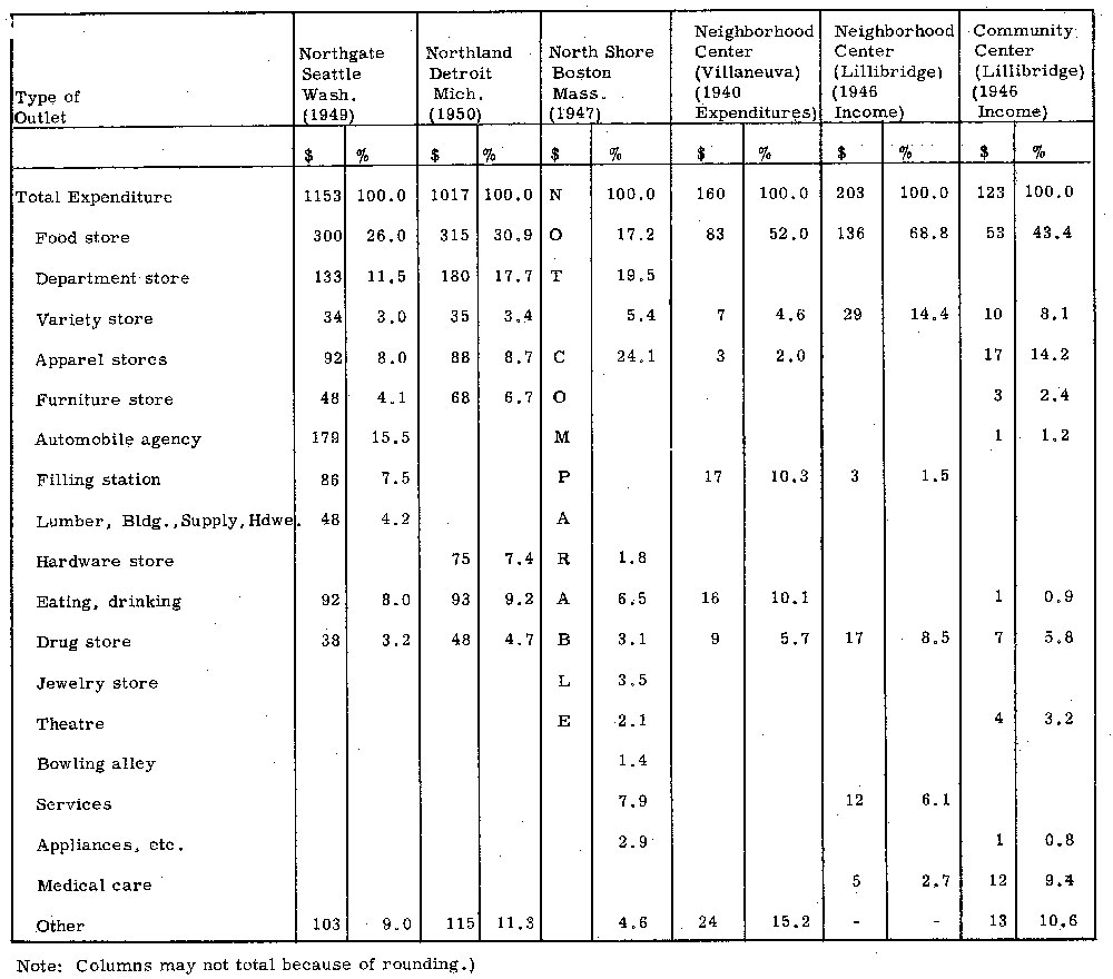
Table XIII shows several examples of a translation from total expenditures into expenditures by type of outlet. It will be seen that there is no great consistency among the various analyses. It should be pointed out that the data for the North Shore Center in Boston are applicable to the shopping center and not to the entire population in the market area. These figures are really a step beyond the others in that the discounts for competition have already been applied.
TABLE XII
PER CENT OF CONSUMER EXPENDITURE FOR CURRENT CONSUMPTION, 1950
Averages and extremes for 16 cities
| Minimum | Maximum | ||||
|---|---|---|---|---|---|
| Expenditure Group | Average %* | %* | City | %* | City |
| Housing, fuel, utilities household operation | 20.6 | 17.2 | Ravenna, Ohio | 23.2 | Boston, Mass. |
| House furnishings & equipment | 6.9 | 5.7 | Boston, Mass. Lynchburg, Va. |
8.7 | Charleston, W.Va. Ravenna, Ohio |
| Food | 29.3 | 26.9 | Minneapolis, Minn. | 31.5 | Philadelphia, Pa. Boston, Mass. |
| Alcoholic drinks & tobacco | 3.4 | 2.3 | Charleston, W.Va. | 4.5 | Lynchburg, Va. |
| Personal care | 2.3 | 2.0 | New York, N.Y. Portland, Ore. Pulaski, Va. |
2.9 | Kansas City, Mo. |
| Clothing | 11.8 | 10.3 | Portland, Ore. | 12.8 | Charleston, W.Va. |
| Medical care | 5.3 | 4.7 | Boston, Mass. Pittsburgh, Pa. Madill, Okla. |
6.4 | Lynchburg, Va. |
| Recreation, reading, education | 6.0 | 4.0 | Lynchburg, Va. | 6.9 | New York, NY |
| Transportation | 13.6 | 8.4 | New York, N.Y. | 16.8 | Portland, Ore. |
| Miscellaneous | 1.3 | 0.7 | Ravenna, Ohio | 2.3 | Madill, Okla. |
* Will not total 100%.
Source: Monthly Labor Review, August, 1952
TABLE XIII
PER CAPITA RETAIL EXPENDITURE BY TYPE OF OUTLET
CONCLUSION
It will be evident that a determination of market potentials for a shopping center requires a great deal of judgment. As mentioned before, economic analyses are notoriously conservative. The analysis of potential sales at the Bon Marche department store in Northgate forecast a total of less than $5 million. The actual sales in 1951 were approximately $10 million. It was predicted that the Hecht Company branch department store in Silver Spring would do an annual business of $5 million when it opened in 1947. In 1948, the actual sales were $7.5 million, and the 1951 sales were $12.5 million. These figures are not pointed out to encourage over-optimistic estimates of sales potential. The estimate should remain conservative. However, when land is purchased for a shopping center site on the basis of an economic analysis, it should be remembered that once a shopping center is built and operating, it is virtually impossible to add additional land to the site. Since land is usually one of the smaller cost items, the developer should assure himself that he at least has ample land to take care of a great deal more business than he anticipates.
ENDNOTES
1 For all references, see bibliography at end.
2 An analysis of these two studies will be included in a later report, and the explanation of the wide discrepancy will be given.
Bibliography
The following references are selected for their application to the problem of analyzing market potential. Many of these cover additional aspects of shopping centers, and there are other references on shopping center design which are not included.
I. Books, general articles, data sources:
BAKER, Geoffrey, and FUNARO, Bruno. "Shopping Centers, Architectural Record's Building Types Study Number 152." Architectural Record, August 1949. Pp. 110–135. (Practically all data here are included in the book Shopping Centers: Design and Operation, by the same authors.)
BAKER, Geoffrey, and FUNARO, Bruno, Shopping Centers: Design and Operation. Reinhold Publishing Corporation, New York, 1951. pp. 288. index. ($12.00). (The most complete manual on shopping centers yet published. Seven chapters on analysis, design and operation. Descriptions and analyses, some in more detail than others, of 63 shopping centers.)
BUREAU OF LABOR STATISTICS, U. S. Department of Labor:
Articles in Monthly Labor Review:
(a) "Expenditures of Moderate Income Families: 1934–36 and 1945." Mary C. Nuark, Vol. 66, No.6, June 1946. pp. 622–626. (Birmingham, Alabama; Indianapolis, Indiana; Portland, Oregon.)
(b) "Family Income and Expenditures in 1947." Helen M. Humes. Vol. 68, No.4, April 1949. pp. 389–397. (Manchester, New Hampshire; Richmond, Virginia; Washington, D.C.)
(c) "Family Income and Expenditures: Los Alamos, 1948." Eleanor M. Snyder and Thomas J. Lanahan, Sr. Vol. 69, No.3, September 1949. pp. 247–251.
(d) "Consumer Spending: Denver, Detroit, and Houston, 1948." Vol. 69, No.6, December 1949. pp. 629–639.
(e) "Survey of Consumer Expenditures in 1950." Mary C. Ruark and Abner Hurwitz. Vol. 75, No.2, August 1952. pp. 125–133. (See list of cities following. )
(f) (Data for Milwaukee, Wisconsin; Savannah, Georgia; and Scranton, Pennsylvania, were collected in 1946 and are available in mimeographed sheets from the Bureau.)
Note: Data for the following cities are given in considerable detail in reference (e):
New York, New York
Chicago, Illinois
Los Angeles, California
Philadelphia, Pennsylvania
Boston, Massachusetts
Pittsburgh, Pennsylvania
Minneapolis, Minnesota
Kansas City, Missouri
Portland, Oregon
Canton, Ohio
Charleston, West Virginia
Lynchburg, Virginia
Grand Forks, North Dakota
Ravenna, Ohio
Pulaski, Virginia
Madill, Oklahoma
Data are also given in reference (e) to the following cities, but in less detail:
Baltimore, Maryland
Cleveland, Ohio
Newark, New Jersey
St. Louis, Missouri
San Francisco, California
Atlanta, Georgia
Birmingham, Alabama
Cincinnati, Ohio
Hartford, Connecticut
Indianapolis, Indiana
Louisville, Kentucky
Miami, Florida
Milwaukee, Wisconsin
New Orleans, Louisiana
Norfolk, Virginia
Omaha, Nebraska
Providence, Rhode Island
Scranton, Pennsylvania
Seattle, Washington
Youngstown, Ohio
Albuquerque, New Mexico
Bakersfield, California
Bangor, Maine
Bloomington, Illinois
Butte, Montana
Canton, Ohio
Charleston, South Carolina
Charlotte, North Carolina
Cumberland, Maryland
Des Moines, Iowa
Evansville, Indiana
Huntington, West Virginia
Jackson, Mississippi
Little Rock, Arkansas
Madison, Wisconsin
Middletown, Connecticut
Newark, Ohio
Ogden, Utah
Oklahoma City, Oklahoma
Phoenix, Arizona
Portland, Maine
Salt Lake City, Utah
San Jose, California
Sioux Falls, South Dakota
Tucson, Arizona
Wichita, Kansas
Wilmington, Delaware
Anna, Illinois
Antioch, California
Barre, Vermont
Camden, Arkansas
Cheyenne, Wyoming
Columbia, Tennessee
Cooperstown, New York
Dalhart, Texas
Demopolis, Alabama
Elko, Nevada
Fayetteville, North Carolina
Garrett, Indiana
Glendale, Arizona
Grand Island, Nebraska
Grand Junction, Colorado
Grinnell, Iowa
Laconia, New Hampshire
Lodi, California
Middlesboro, Kentucky
Nanty-Glo, Pennsylvania
Pecos, Texas
Rawlins, Wyoming
Roseburg, Oregon
Salina, Kansas
Sandpoint, Idaho
Santa Cruz, California
Shawnee, Oklahoma
Shenandoah, Iowa
Washington, New Jersey
ELLWOOD, Leon W., and ARMSTRONG, Robert H. "Shops, Stores and Shopping." (In four parts), Appraisal Journal: Part I, January 1952, pp.13–19; Part II, April 1952, pp. 194–205; Part III, July 1952, pp. 294–302; Part IV, October 1952, pp. 473–480. (A thorough analysis of shopping centers, from viewpoint of real estate appraisal. Contains much useful information.)
FOLEY, Donald L. "The Use of Local Facilities in a Metropolis." American Journal of Sociology, Vol. LVI, No.3, November 1950, pp. 238–246. (Sample of 400 families in northwest St. Louis. Reports use of facilities, such as shopping, school, church, movies, etc., that could be classified as "local." Greater "local" use associated with high residential density, among other factors.)
GRUEN, Victor, and SMITH, Lawrence P. "Shopping Centers: the New Building Type." Progressive Architecture, June 1952, pp. 67–109. (Contains history, definitions, outline of planning steps, design, etc. An abbreviated manual. Gruen is an architect and Smith is a real estate economist.)
LILLIBRIDGE, Robert M. "Shopping Centers in Urban Redevelopment." Land Economics, May 1948. pp. 137–160. Bibliography. (Also reprinted in Regional Shopping Centers: Planning Symposium, Rubloff and others.) (The most complete analysis for a neighborhood center yet published.)
REILLY, William J. The Law of Retail Gravitation. William J. Reilly, 285 Madison Avenue, New York, New York, 1931. pp. vi–75. 1931. ($10.00.) (The original exposition of Reilly's Law. Contains tables for calculating influence of two cities.)
RUBLOFF, Arthur, and others. Regional Shopping Centers: Planning Symposium. Robert M. Lillibridge, editor. Chicago Region Chapter, American Institute of Planners, 1006 City Hall, Chicago 2, Illinois, June 1952, pp. 62, Bibliography. ($ 3.00.) (Six papers from a symposium held by the Chicago AIP Chapter, some better than others. Includes Lillibridge article "Shopping Centers in Urban Redevelopment.")
SALES MANAGEMENT "Survey of Buying Power." Sales Management, May 10, 1952. (Covers sales by type of outlet for cities and countries in the United States and Canada.)
SMITH, Lawrence E. "Valuation of Neighborhood Shopping Centers." Appraisal Journal, Vol. XIX, No.4, October 1951, pp. 508–517. (Case study of a Cleveland center having about 125,000 square feet of stores. Excellent detail.)
STANDARD RATE AND DATA SERVICE, Consumer Markets. (Covers sales by type of outlet for counties and cities over 5,000 population.)
STEIN, Clarence S., and BAUER, Catherine. Store Buildings and Neighborhood Shopping Centers. (Reprinted from Architectural Record, February 1934) with addenda by National Association of Housing Officials, Chicago, 1934. pp. 17. (One of the earliest published analyses of the modern shopping center. Based on experience in planning for Radburn.)
TANNEY, William W. "Super Markets – Data Program." Appraisal Journal, Vol. XVIII, No.4, October 1950. pp. 431–439. (Results of a survey of 60 stores in Detroit and southeastern Michigan. Shows land cost, building cost, rental, size, parking, etc.)
U.S. DEPARTMENT OF AGRICULTURE. How Families Use Their Incomes. Miscellaneous Publication No. 653. U. S. Department of Agriculture, U. S. Government Printing Office, 1948. pp. 64. For sale by Superintendent of Documents, Washington 25, D. C. (30¢.) (Includes both city and farm family expenditures. An excellent study, but not specific for individual cities.)
URBAN LAND INSTITUTE. Community Builders Handbook. Prepared by Community Builders' Council of Urban Land Institute, Washington, D. C., 1947. (Third revised edition 1950.) pp. 205. Index. ($12.00.) (Contains a section on shopping centers. Discusses neighborhood and community centers. Excellent manual.)
URBAN LAND INSTITUTE. Shopping Centers: An Analysis. Technical Bulletin No. 11, Urban Land Institute, Washington, D. C. 1949. pp. 48. ($5.00.) (General discussion of shopping centers and individual analysis of 17 centers.)
VILLANEUVA, Marcel. Planning Neighborhood Shopping Centers. National Committee on Housing, 1 Madison Avenue, New York 10, New York. 1945. pp. 34. ($1.00.) (A study using purchasing power as a yardstick in developing commercial centers. While the figures may be out of date, the methodology is still good.)
WELCH, Kenneth C. "Regional Shopping Centers." Architectural Record's building types study No. 172. Architectural Record, March 1951. pp. 121–143. (Contains an analysis of proposed Sylvania-Douglas center in Toledo, Ohio.)
II. Published analyses of sales data on shopping centers:
BROADWAY-CRENSHAW CENTER, Los Angeles, California. (See BAKER and FUNARO (1951) p. 175.)
CAMERON VILLAGE CENTER, Raleigh, North Carolina. (See BAKER and FUNARO (1951) p. 151.)
CLEARVIEW SHOPPING CENTER, Princeton, New Jersey. (See BAKER and FUNARO (1951) p. 196.)
EVERGREEN PARK SHOPPING CENTER, Chicago, Illinois. (See RUBLOFF above.)
LIDO SHOPPING CENTER, Newport Harbor, California. (See BAKER and FUNARO 1951) p. 275).
NORTH SHORE CENTER, Beverly, Massachusetts. Architectural Forum, 1947. (This is apparently the preliminary analysis for Shoppers' World.)
NORTHGATE CENTER, Seattle, Washington. (See BAKER and FUNARO (1951) p. 219.)
NORTHLAND CENTER, Detroit, Michigan. Progressive Architecture, June 1952, p. 79. (See also BAKER and FUNARO (1951) p. 268.)
PARK FOREST SHOPPING CENTER, Park Forest, Illinois. (See BAKER and FUNARO (1951) p. 268.)
RADBURN, NEW JERSEY. (See STEIN and BAUER above.)
SHOPPERS' WORLD, Framingham, Massachusetts. Architectural Forum, December 1951, p. 181.
SYLVANIA-DOUGLAS CENTER, Toledo, Ohio. Architectural Record, March 1951. p. 121.
*Copyright, American Society of Planning Officials, November, 1952.